Bayesian Linear Regression
Null Models
So far, we’ve really only been interested in 1 variable problems (the proportion of twitter accounts that are bots). What is the most common frequentist approach to for estimating $p$? Maximum Likelihood Estimation.
The Frequentist Way
$$\color{red}{L(\text{data}|p)} = \prod_{i=1}^n p^{x_i} (1 - p)^{1-x_i}$$
$$\color{red}{L(\text{data}|p)} = p^{\sum x_i} (1 - p)^{n- \sum x_i}$$
$$l(\text{data}|p) = \ln p \sum x_i + \ln (1-p) \left(n- \sum x_i \right) $$
In our simple case, 2 accounts were sampled and only one was authentic. $\sum x_i = 1$
$$l(\text{data}|p) = \ln p + \ln (1-p)$$
We want to maximize this. For what value of $p$ is this maximized?
$$\frac{d}{dp} l(\text{data}|p) = \frac{1}{p} - \frac{1}{1-p} = 0$$
$$ \frac{1}{p} = \frac{1}{1-p}$$
$$ {p} = {1-p}$$
$$ \hat{p} = \frac{1}{2}$$
The Bayesian Way
$$\pi(p|\text{data}) \propto \color{red}{L(\text{data}|p)} \pi(p)$$
In our example,
$$B \vert p \sim \text{Bernoulli}(p)$$
$$p \sim \text{Uniform}(0, 1)$$
$$\pi(p|X = 1) = 6p(1-p)$$
Remark: What is the mean of this distribution?
$$\mathbb{E}[\pi(p\vert X = 1)] = \int_0^1 p * 6p(1-p) dp$$
$$\mathbb{E}[\pi(p\vert X = 1)] = \frac{1}{2}$$
Two parameters does not mean two variables
Consider the normal distribution, which is governed by two parameters.
$$X \sim \text{Normal}(\color{blue}{\mu}, \color{green}{\sigma^2})$$
Adding a Predictor
import pandas as pd
import numpy as np
import matplotlib.pyplot as plt
import seaborn as sns
from scipy.stats import norm
df = pd.read_csv('statistical-rethinking/data/howell.csv', delimiter = ';')
df.plot('weight', 'height', kind = 'scatter')
plt.show()
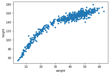
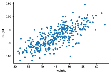
df[df.age >= 18].plot('weight', 'height', kind = 'scatter')
plt.show()
Linear Model Structure
$$\text{Height}_i = \beta_0 + \beta_1\text{Weight}_i + \epsilon \quad \epsilon \sim \text{Normal}(0, \sigma^2)$$
We want to solve for the parameters $\beta_0, \beta_1$
Solve the Frequentist Way
Ordinary Least Squares
$$\min_{\beta_0, \beta_1} \sum_{i=1}^n (h_i - (\beta_0 + \beta_1 w_i))^2$$
Maximum Likelihood Estimation
$$L(\text{height}|\beta_0, \beta_1, \sigma^2, \text{weight}) = \prod_{i=1}^n \frac{1}{\sigma^2\sqrt{2\pi}} \exp \bigg\{-\frac{(h_i - (\beta_0 + \beta_1 w_i))^2}{2\sigma^2} \bigg\}$$
Solutions:
$$\hat \beta_0 = \bar h - \hat \beta_1 \bar w$$
$$\hat \beta_1 = \frac{\sum_{i=1}^n(w_i - \bar w)(h_i - \bar h)}{\sum_{i=1}^n (w_i - \bar w)^2}$$
adults = df[df.age >= 18]
adults = adults.sort_values('weight').reset_index(drop = True)
adults.head()
| height | weight | age | male | |
|---|---|---|---|---|
| 0 | 143.510 | 31.071052 | 18.0 | 0 |
| 1 | 141.605 | 31.524644 | 19.0 | 1 |
| 2 | 142.240 | 31.666391 | 36.0 | 0 |
| 3 | 136.525 | 31.864838 | 65.0 | 0 |
| 4 | 146.050 | 31.864838 | 44.0 | 0 |
weight = adults.weight.to_numpy()
height = adults.height.to_numpy()
Solve for $\beta_1$
w_bar = weight.mean()
h_bar = height.mean()

beta_1 = np.sum((weight - w_bar) * (height - h_bar)) / np.sum((weight - w_bar) ** 2)
beta_1
0.9050291086266476
Solve for $\beta_0$
# some stuff #

beta_0 = h_bar - beta_1 * w_bar
beta_0
113.8793936068935
Plot results
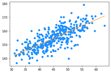
plt.scatter(weight, height, color = 'dodgerblue')
plt.plot(weight, beta_0 + beta_1 * weight, color = 'darkorange')
plt.show()
Solve the Bayesian Way
$$h_i \sim \text{Normal}(\mu, \sigma^2)$$
$$\mu = \beta_0 + \beta_1 (w_i - \bar w)$$
$$\beta_0 \sim \text{Normal}(150, 10)$$
$$\beta_1 \sim \text{Normal}(0, 10)$$
$$\sigma^2 \sim \text{Exp}(1)$$
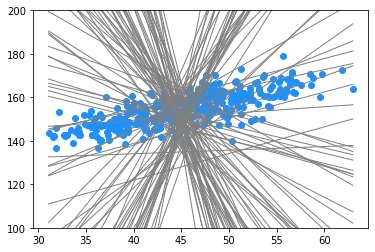
beta_0s = np.random.normal(size = 100, loc = 150, scale = 10)
beta_1s = np.random.normal(size = 100, loc = 0, scale = 10)

for b0, b1 in zip(beta_0s, beta_1s):
    plt.plot(weight, b0 + b1 * (weight - weight.mean()), color = 'grey', linewidth = 1)
plt.ylim(100, 200)
plt.scatter(weight, height, color = 'dodgerblue')
plt.show()
$$h_i \sim \text{Normal}(\mu, \sigma^2)$$
$$\mu = \beta_0 + \beta_1(w_i - \bar w)$$
$$\beta_0 \sim \text{Normal}(150, 10)$$
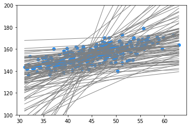
$$\beta_1 \sim \text{Log-Normal}(0, 1)$$
$$\sigma^2 \sim \text{Exp}(1)$$
beta_0s = np.random.normal(size = 100, loc = 150, scale = 10)
beta_1s = np.random.lognormal(size = 100, mean = 0, sigma = 1)

for b0, b1 in zip(beta_0s, beta_1s):
    plt.plot(weight, b0 + b1 * (weight - weight.mean()), color = 'grey', linewidth = 1)
plt.ylim(100, 200)
plt.scatter(weight, height, color = 'dodgerblue')
plt.show()
def prior(b0, b1, s):


    b0_prior = norm.pdf(x = b0, loc = 150, scale = 10)
    b1_prior = np.exp(norm.pdf(x = b1, loc = 0, scale = 1))
    s_prior  = np.exp(-s)
    ######################

    # log probability transforms multiplication to summation
    return np.log(b0_prior) + np.log(b1_prior) + np.log(s)

def likelihood(b0, b1, s):


    mu = b0 + b1 * (weight - weight.mean())
    likelihoods = norm(loc = mu, scale = s).pdf(x = height)
    ######################

    # log probability transforms multiplication to summation
    return np.sum(np.log(likelihoods))

def posterior(b0, b1, s):

    return likelihood(b0, b1, s) + prior(b0, b1, s)

def proposal(b0, b1, s):

    b0_new = np.random.normal(loc = b0, scale = 0.5)
    b1_new = np.random.normal(loc = b1, scale = 0.5)
    s_new  = max(np.random.uniform(low = s - 0.1, high = s + 0.1), 0.01)

    return b0_new, b1_new, s_new
steps = 10000
b0_steps = np.zeros(steps)
b1_steps = np.zeros(steps)
sigma_steps = np.zeros(steps)

b0_steps[0]     = 155
b1_steps[0]     = 1
sigma_steps[0]  = 3

for step in range(1, steps):

    b0_old     = b0_steps[step - 1]
    b1_old     = b1_steps[step - 1]
    sigma_old = sigma_steps[step - 1]

    b0_new, b1_new, s_new = proposal(b0_old, b1_old, sigma_old)

    # Use exp to restore from log numbers
    accept_ratio = np.exp(posterior(b0_new, b1_new, s_new) - posterior(b0_old, b1_old, sigma_old))

    if np.random.uniform(0, 1) < accept_ratio:
        b0_steps[step], b1_steps[step], sigma_steps[step]  = b0_new, b1_new, s_new

    else:
        b0_steps[step], b1_steps[step], sigma_steps[step]  = b0_old, b1_old, sigma_old
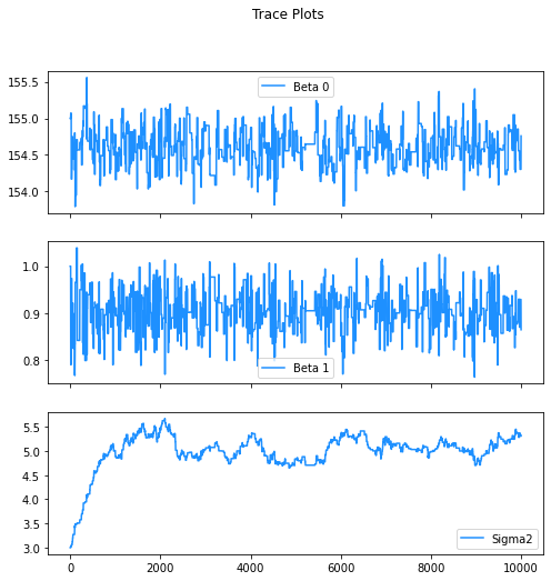
fig, (ax1, ax2, ax3) = plt.subplots(3, figsize = (8, 8), sharex = True)
fig.suptitle('Trace Plots')
sns.lineplot(ax  = ax1, x = range(steps), y = b0_steps, label = "Beta 0", color = "dodgerblue")
sns.lineplot(ax  = ax2, x = range(steps), y = b1_steps, label = "Beta 1", color = "dodgerblue")
sns.lineplot(ax  = ax3, x = range(steps), y = sigma_steps, label = "Sigma2", color = "dodgerblue")
<AxesSubplot:>
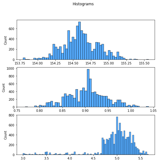
fig, (ax1, ax2, ax3) = plt.subplots(3, figsize = (8, 8))
fig.suptitle('Histograms')
sns.histplot(ax  = ax1, x = b0_steps, label = "Beta 0", color = "dodgerblue")
sns.histplot(ax  = ax2, x = b1_steps, label = "Beta 1", color = "dodgerblue")
sns.histplot(ax  = ax3, x = sigma_steps, label = "Sigma2", color = "dodgerblue")
<AxesSubplot:ylabel='Count'>
b1_steps.mean(), beta_1
(0.9030567272623151, 0.9050291086266476)
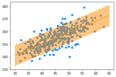
89% Confidence Interval for Heights
n = 5000
weights = np.linspace(30, 65, len(weight))
lower_89 = np.zeros(len(weight))
upper_89 = np.zeros(len(weight))

for i, w in enumerate(weights):
    mu = b0_steps[-n:] + b1_steps[-n:] * (w - weight.mean())
    sigma = sigma_steps[-n:]
    heights = np.random.normal(size = n,
                               loc = mu,
                               scale = sigma)

    lower_89[i], upper_89[i] = np.quantile(heights, q = (0.055, 1 - 0.055))
plt.scatter(weight, height, color = 'dodgerblue')
plt.plot(weights, b0_steps.mean() + b1_steps.mean() * (weights - weight.mean()), color = "darkorange")
plt.fill_between(weights, upper_89, lower_89, color = "darkorange", alpha = 0.5)
plt.show()
Prediction
What is the expected height and 89% credible interval for someone who weighs 50kg?
n = 1000
mu = b0_steps.mean() + b1_steps.mean() * (50 - weight.mean())
sigma = sigma_steps.mean()
height_dist = np.random.normal(size = n, loc = mu_dist, scale = sigma)
sns.histplot(x = height_dist, color = "dodgerblue")
<AxesSubplot:ylabel='Count'>
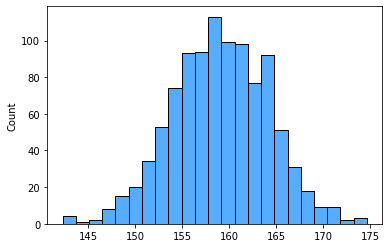
Expected Value?
height_dist.mean()
159.06495731205368
89% Credible Interval
np.quantile(height_dist , q = (0.055, 1 - 0.055))
array([151.00466849, 166.94544509])
Appendix
MLE for Normal Distribution
$$\color{red}{L(\text{data}|\color{blue}{\mu}, \color{green}{\sigma^2})} = \prod_{i=1}^n \frac{1}{\color{green}{\sigma^2}\sqrt{2\pi}} \exp \bigg\{-\frac{(x_i - \color{blue}{\mu})^2}{2\color{green}{\sigma^2}} \bigg\}$$
$$\color{red}{L(\text{data}|\color{blue}{\mu}, \color{green}{\sigma^2})} \propto \frac{1}{\color{green}{\sigma}^{2n}} \exp \bigg\{-\frac{\sum_{i=1}^n(x_i - \color{blue}{\mu})^2}{2\color{green}{\sigma^2}} \bigg\}$$
$$l(\text{data}|\color{blue}{\mu}, \color{green}{\sigma^2}) \propto -2n \ln \color{green}{\sigma} -\frac{\sum_{i=1}^n(x_i - \color{blue}{\mu})^2}{2\color{green}{\sigma^2}}$$
We want to maximize this. What values of $\color{blue}{\mu}, \color{green}{\sigma^2}$ will this be maximized?
$$\frac{d}{d\color{blue}{\mu}} l(\text{data}|\color{blue}{\mu}, \color{green}{\sigma^2}) \propto \frac{\sum_{i=1}^n(x_i - \color{blue}{\mu})}{2\color{green}{\sigma^2}} = 0$$
$$\sum_{i=1}^n(x_i - \color{blue}{\mu}) = 0$$
$$\sum_{i=1}^n(x_i) - n\color{blue}{\mu} = 0$$
$$ \boxed{ \color{blue}{\hat\mu} = \frac{1}{n} \sum_{i=1}^n x_i} = \text{"Sample mean"}$$
$$\frac{d}{d\color{green}{\sigma}} l(\text{data}|\color{blue}{\mu}, \color{green}{\sigma}) \propto \frac{-n}{\color{green}{\sigma}} +\frac{\sum_{i=1}^n(x_i - \color{blue}{\mu})^2}{\color{green}{\sigma^3}} = 0$$
$$-n +\frac{\sum_{i=1}^n(x_i - \color{blue}{\mu})^2}{\color{green}{\sigma^2}} = 0$$
$$n = \frac{\sum_{i=1}^n(x_i - \color{blue}{\mu})^2}{\color{green}{\sigma^2}}$$
$$\boxed{\color{green}{\hat \sigma^2} = \frac{\sum_{i=1}^n(x_i - \color{blue}{\hat \mu})^2}{n}} = \text{"Population variance"}$$
Sources
Statistical Rethinking - Richard McElreath